TTT-Discover: Learning to Discover at Test Time
This post is part of the AI-Driven Research for Systems (ADRS) blog series, where we explore how AI can be applied to systems research. We feature exciting work on TTT-Discover this week!
TTT-Discover keeps training the LLM on a single test problem instead of prompting a frozen one. AlphaEvolve and OpenEvolve stuff past attempts into better prompts; the weights never move. TTT-Discover runs RL on the test problem itself, using an objective built for discovery rather than average performance. Everything runs on the open gpt-oss-120b for a few hundred dollars a problem.
📄 Paper · 💻 Code · 🔍 Webpage & Demo
More from ADRS:
- ✍️ Previous Blogs: https://ucbskyadrs.github.io/
- 📝 ADRS Paper: https://arxiv.org/abs/2510.06189
- 👩💻 ADRS Code: github.com/UCB-ADRS/ADRS
- 💬 Join us: join.slack.com/t/adrs-global and Discord
- Follow us: x.com/ai4research_ucb
The Problem
Science and engineering are full of problems where the goal is to beat the best known result: a faster GPU kernel, a tighter bound on an open math problem, a higher-scoring scheduling algorithm. The current best already exists, at the top of a leaderboard or in a 2016 paper, and anything short of beating it counts for nothing. These are discovery problems.
They are hard for LLMs almost by definition. The record-beating solution appears in no training set, so the model has to generalize past everything it has seen. The standard workaround is search. Methods like AlphaEvolve and OpenEvolve sample a frozen model thousands of times, store the best attempts in a buffer, and feed them back into ever-richer prompts. The prompts and the solution tend to improve, but the model never does. Yet those attempts are exactly the data the problem was missing: hundreds of solutions to this specific out-of-distribution problem, which existed nowhere before the search started. Putting them in a prompt is the weakest way to use them. The stronger way is to train on them.
The catch is that standard RL is built for the wrong goal. It maximizes expected reward, because in normal RL the policy is the product: it will be deployed and needs to be reliably good. In discovery the policy is disposable. All that matters is that it produces one record-beating solution, even if 999 out of 1,000 attempts fail, and average-reward training would smooth that one-in-a-thousand behavior away. Restarting every attempt from a blank slate also caps how much structure a single attempt can build.
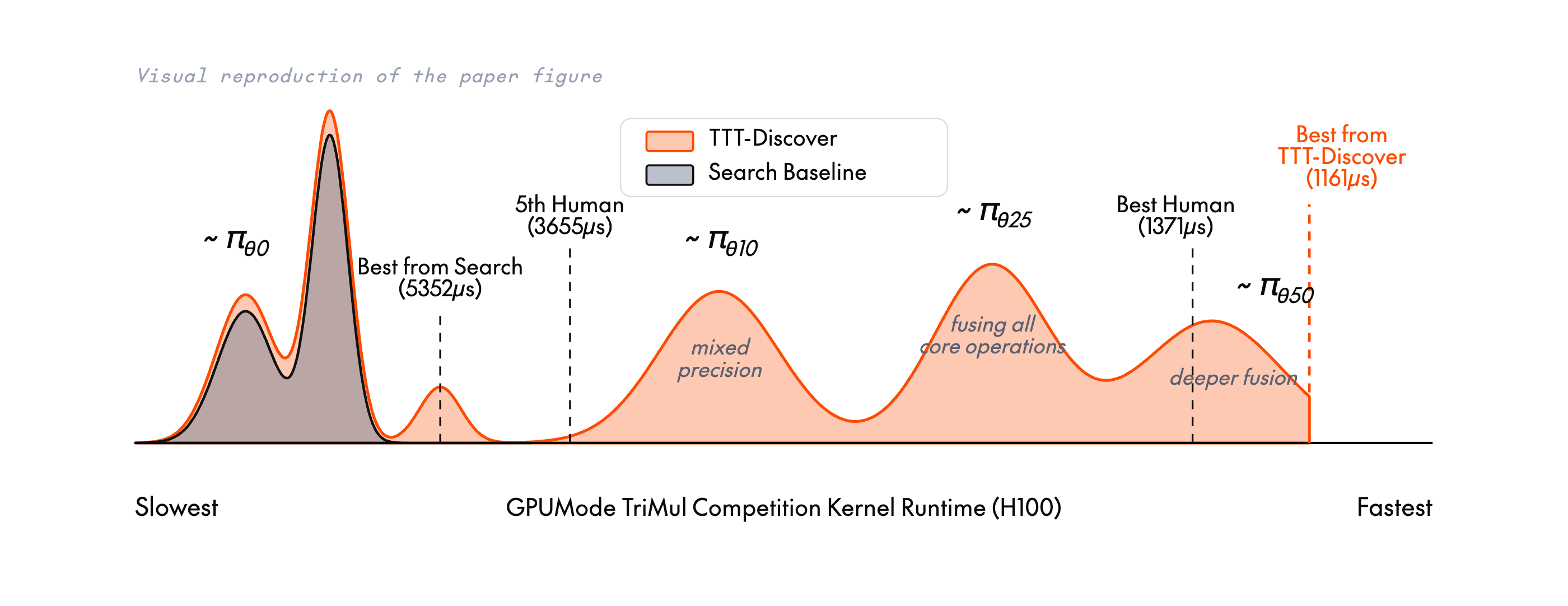
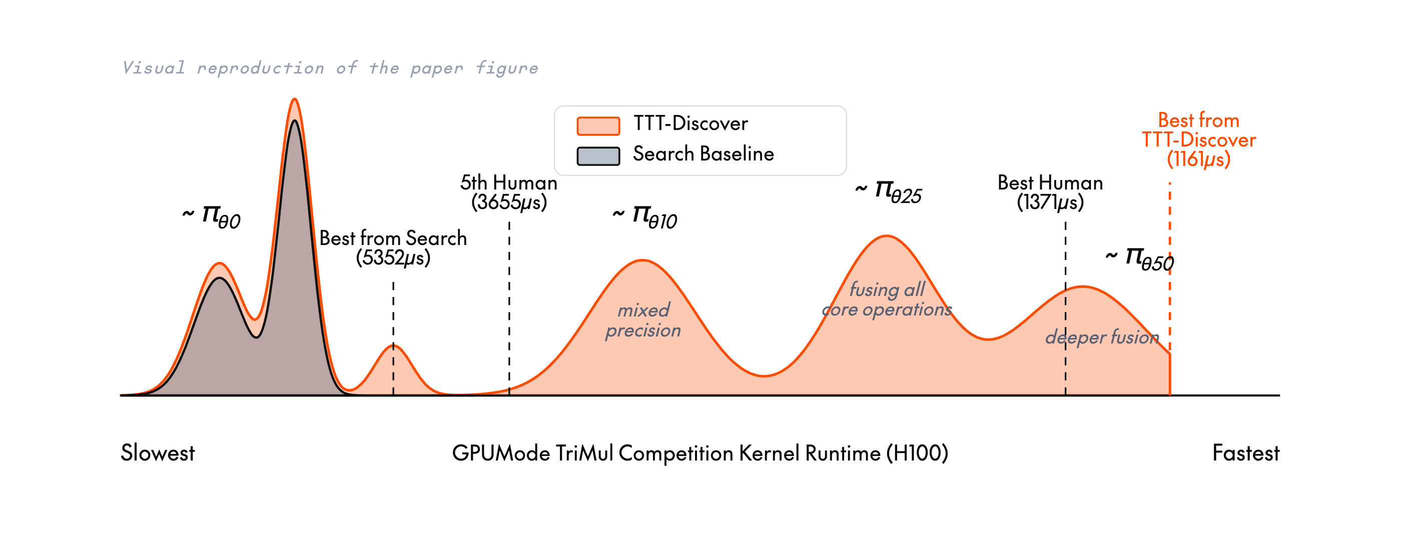
On TriMul, a GPU-kernel task from the GPUMode competition (runtime in µs, lower is better), best-of-N sampling with the same model and the same 25,600 attempts, no training at all, produced 5,352 µs.
TTT-Discover keeps the training and fixes the objective. It runs RL on the single test problem, with a learning objective that chases the maximum rather than the mean, and a reuse rule that keeps building on the most promising solutions. Everything runs on the open gpt-oss-120b for a few hundred dollars a problem.
Entropic Objective and PUCT reuse
Two changes turn standard RL into a discovery method.
The entropic objective. Standard RL maximizes expected reward:
max_θ E_{y ~ π_θ}[R(y)]
TTT-Discover instead maximizes an entropic objective where rollouts are weighted exponentially by reward with a parameter β:
max_θ log E_{y ~ π_θ}[e^{β R(y)}]
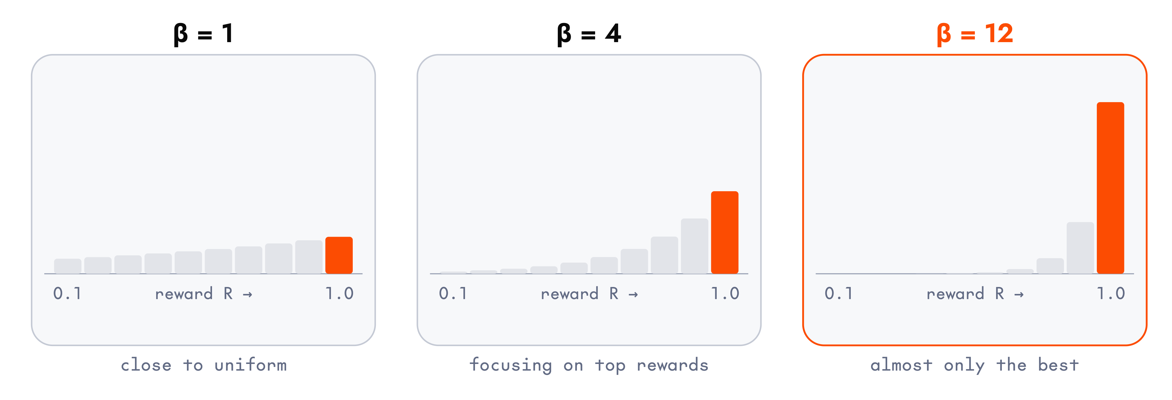
As β gets smaller we recover the standard expected-reward objective; as β grows the update is dominated by the highest-reward rollouts, so the gradient chases the max rather than the mean. In practice a fixed β is brittle, so it's set adaptively per state (see the paper for this detail).
Here a figure that describes the intuition behind the use of β:
PUCT reuse. To extend the effective horizon and balance exploring new states against re-expanding promising ones, states are selected AlphaZero-style:
a* = argmax_a Q(s,a) + c · P(s,a) · √N(s) / (1 + N(s,a))
The change is in Q. AlphaZero sets Q(s,a) to the average reward of simulations through the node; here it's the best descendant's reward:
Q(s,a) = max_{y ∈ desc(s,a)} R(y)
So a kernel that once seeded a faster kernel keeps its credit, however many duds came alongside.
The paper describes four applications of TTT-Discover to kernel engineering, math, algorithm engineering and biology. Here will give an overview of the first two. For Kernel Engineering, we focus on optimizing the TriMul kernel (an operation important in models like AlphaFold), for math we focus on two combinatorics tasks that AlphaEvolve tackled back in 2025: the Erdős minimum overlap and the first autocorrelation inequality.
Kernel Engineering
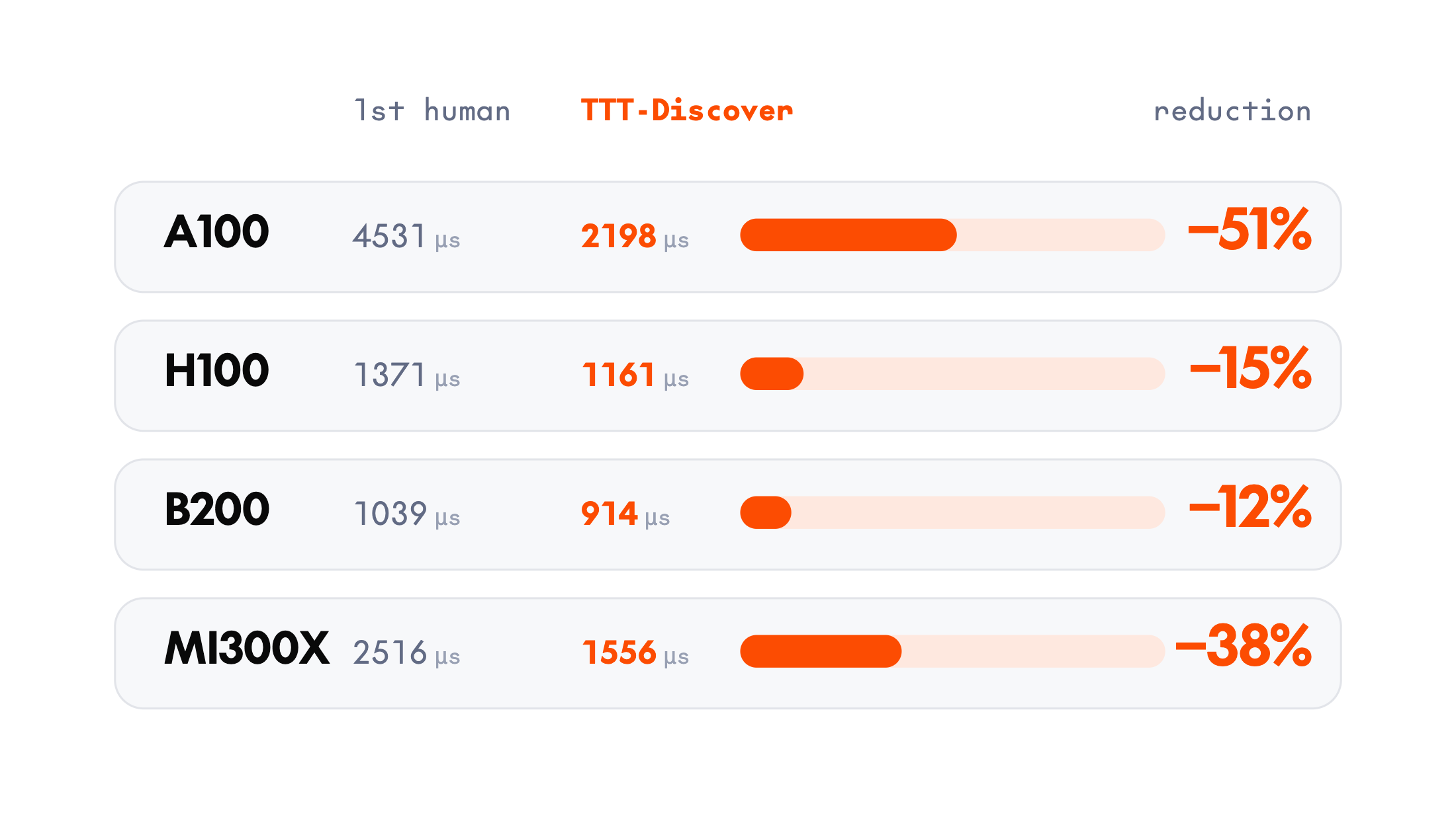
At the time of submission, the TriMul kernels found by TTT-Discover beat the top human on all four GPU types. A100 went from 4,531 μs to 2,198, H100 from 1,371 to 1,161. Training only ever timed kernels on H100s, so the A100 result came from generalization the reward function never asked for.
The winning kernel treats the problem as memory bound and fuses three groups of operations the reference runs separately: the input LayerNorm, the sigmoid and elementwise multiply in the input gate, and the output LayerNorm with the output gate. For the O(N³) matmul it converts to FP16 and hands the work to cuBLAS. GPUMode's organizers called this the same strategy the best humans use, executed better, since most human submissions fuse fewer of the complex operators.
Two Problems in Additive Combinatorics
We tackle two math problems that also appeared in the AlphaEvolve paper.
The first is Erdős' minimum overlap problem, open since 1955. Split the numbers 1 through 2n into two equal piles, count the pairs separated by each gap k, and find the split that keeps the most common gap as rare as possible. Call that count M(n); the question is what M(n)/n tends to as n grows. The best human bound, due to Haugland in 2016, stood at 0.380927.
The second is the first autocorrelation inequality. Convolve a nonnegative function with itself: the peak of that self-convolution always stays above C₁ times the square of the function's mass. Any function with a flat enough peak certifies a lower ceiling on C₁, so the search is for such a function.
Both reduce to the same kind of optimization: over step functions of bounded norm, minimize the largest value a correlation reaches. A result of Swinnerton-Dyer lets a density function stand in for the Erdős partition, and whatever construction comes out certifies its bound on its own. No proof needed beyond evaluating the function.
TTT-Discover set the record on both.
On the inequality it reached 1.50287, past ThetaEvolve's 1.50314 (lower is better). The gap between the methods is larger than the gap between the numbers: ThetaEvolve refined AlphaEvolve's 1,319-piece construction, while TTT-Discover started from random functions and built a 30,000-piece one from scratch.
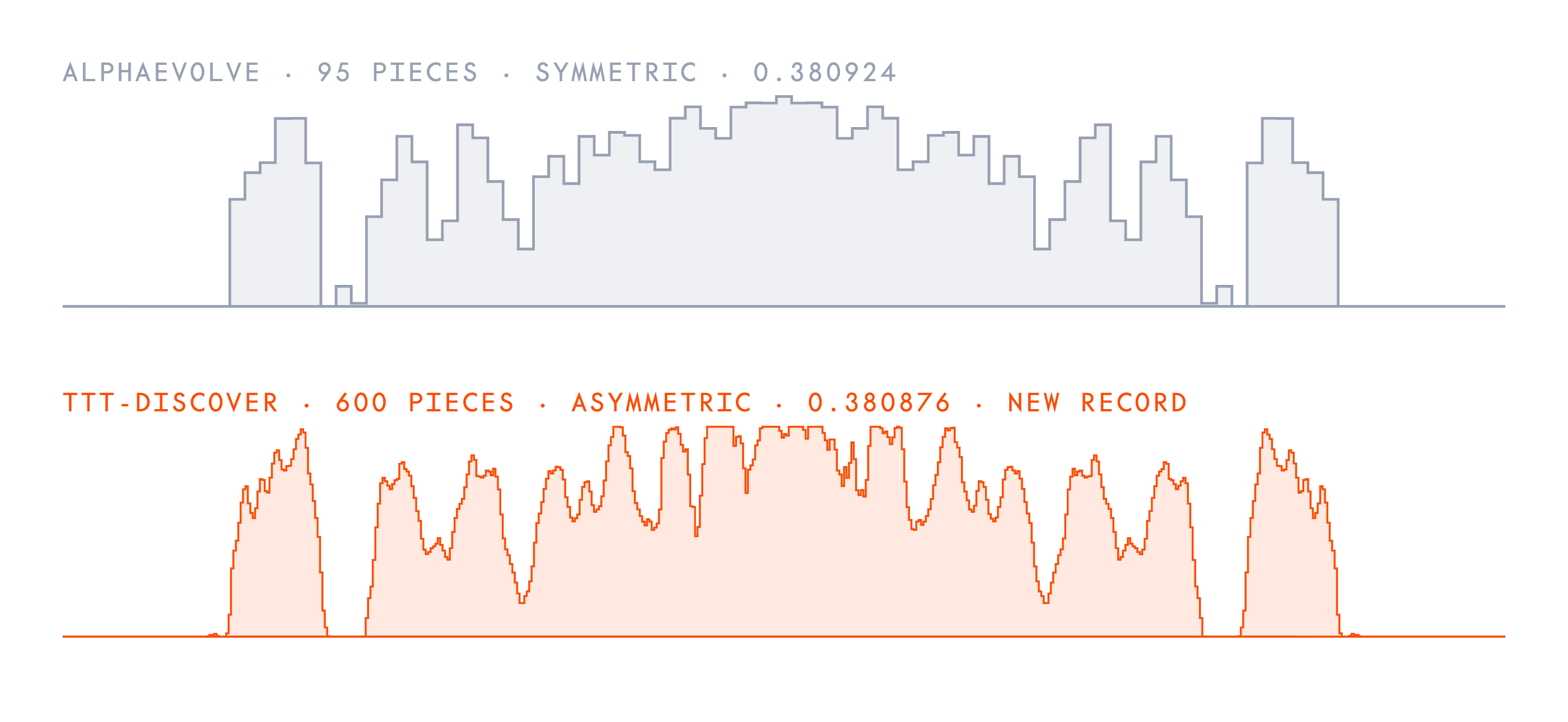
On Erdős, AlphaEvolve had moved Haugland's bound to 0.380924. TTT-Discover reached 0.380876, an improvement sixteen times larger than AlphaEvolve's own step. The 600-piece construction also came out asymmetric. Every earlier record holder, Haugland's 51-piece and AlphaEvolve's 95-piece included, was symmetric.
Conclusion
The comparison carrying the paper is TTT-Discover against Best-of-25,600. Same model, same rollout count, same sampling budget. Whether the weights move is the only variable, and it decides every result above. The same recipe, unchanged, set records in kernel engineering, combinatorics, and algorithm engineering, that frontier-model pipelines had held for a while.
Try It Out
TTT-Discover is straightforward to use! First, define your problem and environment
from ttt_discover import Environment, BaseRewardEvaluator, State, DiscoverConfig, discover

# Define your reward function
class YourReward(BaseRewardEvaluator):

    def get_reward(self, code: str, state: State) -> float:
        # ...add logic here for computing reward

        return {
            "reward": reward,
            "correctness": 1.0,
            "raw_score": raw_score,
            "msg": f"Success; raw_score={raw_score}",
            "result_construction": [], # Could reuse
            "stdout": "", # No stdout
        }

class YourEnv(Environment):
    reward_function = YourReward
    state_type = State # You may define your own state if you wish

    def get_question(self) -> str:
        state_ctx = self.initial_state.to_prompt(100, metric_name="performance")

        return f"""You are an expert mathematician specializing in combinatorial problems and computational geometry. Your task is to ... {state_ctx}."""
Then, just train the model!
config = DiscoverConfig(
    env_type=YourEnv,
    experiment_name="test-run",
    wandb_project="",
)

# Run discovery
discover(config)
Citation
@article{ttt-discover2026,
  title   = {Learning to Discover at Test Time},
  author  = {Yuksekgonul, Mert and Koceja, Daniel and Li, Xinhao
             and Bianchi, Federico and McCaleb, Jed and Wang, Xiaolong
             and Kautz, Jan and Choi, Yejin and Zou, James
             and Guestrin, Carlos and Sun, Yu},
  journal = {ICML},
  year    = {2026}
}
Contribute to the ADRS Blog Series!
The AI-Driven Research Systems (ADRS) initiative is an open, collaborative effort to explore how AI can accelerate scientific discovery itself, from evolving algorithms to optimizing real-world systems.
If you've built, optimized, or experimented with AI-driven research tools, we'd love to hear from you. Share your experiences, insights, or case studies with us in the ADRS Blog Series.
👉 Reach out to us via email: ucbskyadrs@gmail.com
💬 Join us: join.slack.com/t/adrs-global and Discord