Automating Algorithm Discovery: A Case Study in Kernel Generation with Datadog BitsEvolve
This post is part of the AI-Driven Research for Systems (ADRS) blog series, where we explore how AI can be applied to systems research. We feature exciting work from Datadog this week!
In this blog post, we examine the problem of generating production-ready, optimized GPU code from an evolutionary search perspective. Specifically, we share results from BitsEvolve, an ADRS framework built at Datadog. BitsEvolve targets various modalities ranging from optimizing hotspots in CPU-bound code to policy/configuration tuning for applications like inference serving frameworks (e.g. vLLM), Load Balancers, Garbage Collectors and more. Through profile guidance and robust evaluation mechanisms, we show how BitsEvolve-generated code can outperform compiled models, achieving speedups of up to 1.6x with reasonable search costs.
- ✍️ Previous Blogs: https://ucbskyadrs.github.io/
- 🚀 Previous BitsEvolve blog post: https://www.datadoghq.com/blog/engineering/self-optimizing-system/
- 📝 ADRS Paper: https://arxiv.org/abs/2510.06189
- 👩💻 ADRS Code: github.com/UCB-ADRS/ADRS
- 💬 Join us: join.slack.com/t and Discord
- Follow us: x.com/ai4research_ucb
The Problem: The Optimization Bottleneck
AI workloads are devouring compute. Across both datacenters and the edge, current trends point to a rising share for GPUs and accelerators. This momentum has also led to rapid maturity and increasing complexity in the GPU software stack. We have evolved from programming GPUs using raw CUDA to a landscape of DSLs and compiler-driven code generation, all with varying levels of efficacy. While well-known examples exist of hand-optimized, performant kernels (relative to peak SOL throughput), such efforts are restricted to a handful of core primitives. Similar to high-performance CPU optimization, the specialized skill set required is rare, and applying it to every niche problem is often not ROI-positive.
Furthermore, given the pace of innovation, the set of possible optimization targets is ever-growing. We must constantly adapt to new GPU architectures and compute capability levels, cost-efficient SKUs, evolving numeric formats (e.g., quantized types, microscaling formats), and shifting model configurations.
So, in the spirit of ADRS, we ask the question: Can we use LLM-based coding agents as our "GPU kernel engineers" to continuously optimize AI/ML workloads?
To explore answers to that question, we built a GPU code optimization and kernel generation flow in BitsEvolve, an agentic optimization system.
Related Work
Automated kernel generation has seen significant interest recently.
- KernelBench provides reference computation graphs across different complexity levels to evaluate correctness and performance on open-weight and proprietary models.
- KernelFalcon takes an agentic approach, combining techniques to achieve 100% correctness on the KernelBench suite.
- KernelLLM explores fine-tuning existing models specifically for GPU kernel generation.
BitsEvolve builds on these ideas but targets a more holistic, production-first approach.
BitsEvolve for GPU Code Optimization

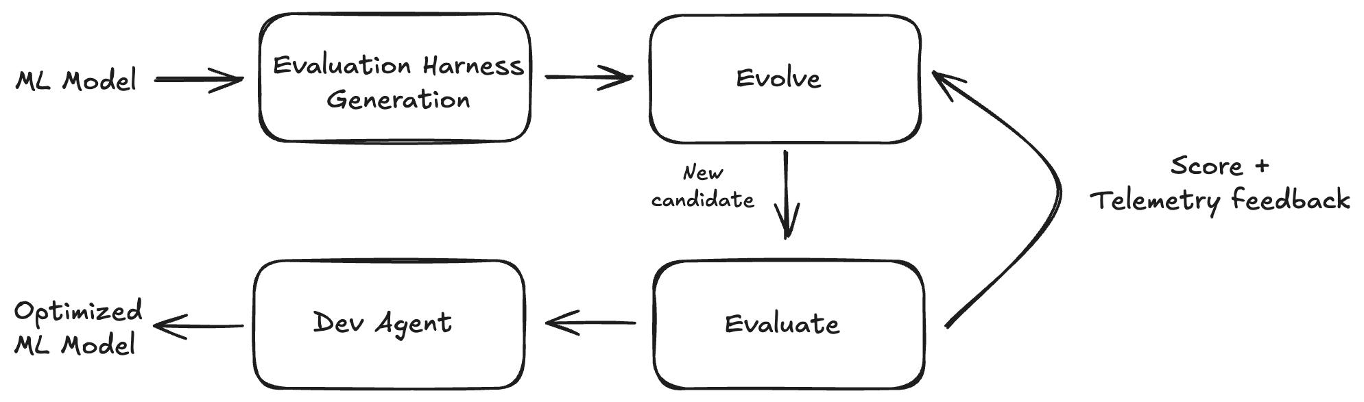
BitsEvolve is an ADRS framework that takes a base ML model (e.g., PyTorch model code) as input, generates an evaluation harness with the model code built in, and executes an LLM-guided evolutionary search as described in our previous Datadog blog post. The result is an optimized model that functions as a drop-in replacement for the original base model.
We build BitsEvolve on top of ShinkaEvolve, adding customizations that we are currently upstreaming (including support for languages like Rust and LLM query streaming). In the core evolutionary loop, we use frontier models: specifically GPT-5, GPT-5.1 (varying reasoning efforts), and Gemini 2.5 Pro (dynamic thinking).
In comparison to the related work mentioned previously, BitsEvolve aims to take a more holistic, layered approach to GPU code optimization. More concretely:
- Modular Evolutionary Search: We retain the core LLM-guided evolutionary search but use modular layers to specialize our approach. For example:
- Flexible Targets: The code generation agent can target raw CUDA, Triton, CuTe, or other vendor-specific DSLs.
- Model Flexibility: The underlying model itself can be a proprietary external model, or a fine-tuned open-weights model.
- Holistic Optimization: Telemetry feedback and whole-model optimization are important anchors for BitsEvolve. We don't restrict ourselves to generating optimized kernels alone but also optimize CPU/GPU synchronization and orchestration overheads, redundant data movement, etc. (see later examples).
- "Merge-Ready" Code: The end goal of a BitsEvolve workflow is deployable production code. This means we need strong validation harnesses guaranteeing correctness, performance, and compatibility.
Real-World Application
We apply this new BitsEvolve workflow to models used internally at Datadog. These models use PyTorch as the model framework and serve production use cases. Our immediate goal was to optimize the forward pass to improve inference serving performance and cost-efficiency.
Shown here is an example fragment from BitsEvolve output. Some notable details:
- The input to the MLP is decomposed into independent branches with partial precomputation
- Dispatching to architecture-specific optimized GEMMs where appropriate
- Fused kernels for remaining operations
- Preallocated output and careful use of views
Optimized Code Example: GliNER Scoring
Reference PyTorch Code
self.out_mlp = nn.Sequential(
            nn.Linear(hidden_size * 3, hidden_size * 4),
            nn.Dropout(dropout),
            nn.ReLU(),
            nn.Linear(hidden_size * 4, 3)  # start, end, score
        )
Optimized Code
tile_s = min(self.tile_s, S)
for b in range(B):
		l1_b = l1[b].contiguous()          # [C, H]
		Pl_b = Pl[b].contiguous()          # [C, 4H]
		Pt_b = Pt[b].contiguous()          # [S, 4H]
    for s0 in range(0, S, tile_s):
        T = min(tile_s, S - s0)

        # 5) Build elementwise-product branch A_tile = l1_b * t1[b, s0:s0+T]
        scales = t1[b, s0:s0+T].contiguous()  # [T, H]
        A_tile = self._kernels.colscale_tile_bf16(l1_b, scales)  # [T, C, H]

        # 6) GEMM: (T*C, H) @ (H, 4H) = (T*C, 4H)
        A2D = A_tile.view(T * C, H).contiguous()
        Ms2D = torch.matmul(A2D, Wmul)  # [T*C, 4H]

        # 7) Fuse (+Pt_tile broadcast +Pl_b broadcast +bias) and ReLU in-place
        Pt_tile = Pt_b[s0:s0+T].contiguous()  # [T, 4H]
        Ms2D = self._kernels.fused_bias_relu_broadcast_inplace(Ms2D, Pt_tile, Pl_b, b1)

        # 8) Final GEMM to logits with bias: (T*C, 4H) @ (4H, 3) + b2
        S2D = torch.addmm(b2, Ms2D, W2T)  # [T*C, 3]

        # 9) Scatter to [B, S, C, 3]
        scores[b, s0:s0+T] = S2D.view(T, C, 3)
// Kernel: out[t, c, h] = l1[c, h] * scales[t, h]
// Shapes: l1 [C, H], scales [T, H], out [T, C, H]
__global__ void bf16_colscale_tile_kernel(
    const __nv_bfloat16* __restrict__ l1,
    const __nv_bfloat16* __restrict__ scales,
    __nv_bfloat16* __restrict__ out,
    int T, int C, int H
){
    int c = blockIdx.x;
    int t = blockIdx.y;
    int tid = threadIdx.x;

    if (c >= C || t >= T) return;

    const __nv_bfloat16* l1_row = l1 + c * H;
    const __nv_bfloat16* scale_row = scales + t * H;
    __nv_bfloat16* out_row = out + (t * C + c) * H;

    for (int h = tid; h < H; h += blockDim.x) {
        float a = __bfloat162float(l1_row[h]);
        float s = __bfloat162float(scale_row[h]);
        out_row[h] = __float2bfloat16_rn(a * s);
    }
}

torch::Tensor colscale_tile_bf16(torch::Tensor l1, torch::Tensor scales) {
    ...
    dim3 block(256);
    dim3 grid(C, T);
    bf16_colscale_tile_kernel<<<grid, block>>>(
        reinterpret_cast<const __nv_bfloat16*>(l1.data_ptr<at::BFloat16>()),
        reinterpret_cast<const __nv_bfloat16*>(scales.data_ptr<at::BFloat16>()),
        reinterpret_cast<__nv_bfloat16*>(out.data_ptr<at::BFloat16>()),
        T, C, H
    );

    return out;
}

// Kernel: Ms2D_inout[(t*C + c), h4] = relu( Ms + Pt[t, h4] + Pl[c, h4] + bias[h4] )
// Shapes: Ms2D [T*C, H4], Pt [T, H4], Pl [C, H4], bias [H4]
__global__ void bf16_fused_bias_relu_broadcast_tile_kernel(
    __nv_bfloat16* __restrict__ Ms2D,           // [T*C, H4]
    const __nv_bfloat16* __restrict__ Pt,       // [T, H4]
    const __nv_bfloat16* __restrict__ Pl,       // [C, H4]
    const __nv_bfloat16* __restrict__ bias,     // [H4]
    int T, int C, int H4
){
    int c = blockIdx.x;
    int t = blockIdx.y;
    int tid = threadIdx.x;

    if (c >= C || t >= T) return;

    __nv_bfloat16* Ms_row = Ms2D + (t * C + c) * H4;
    const __nv_bfloat16* Pt_row = Pt + t * H4;
    const __nv_bfloat16* Pl_row = Pl + c * H4;

    for (int h = tid; h < H4; h += blockDim.x) {
        float m = __bfloat162float(Ms_row[h]);
        float pt = __bfloat162float(Pt_row[h]);
        float pl = __bfloat162float(Pl_row[h]);
        float b = __bfloat162float(bias[h]);
        float v = m + pt + pl + b;
        v = v > 0.f ? v : 0.f;
        Ms_row[h] = __float2bfloat16_rn(v);
    }
}

torch::Tensor fused_bias_relu_broadcast_inplace(
    torch::Tensor Ms2D, torch::Tensor Pt, torch::Tensor Pl, torch::Tensor bias
) {
    ...

    dim3 block(256);
    dim3 grid(C, T);
    bf16_fused_bias_relu_broadcast_tile_kernel<<<grid, block>>>(
        reinterpret_cast<__nv_bfloat16*>(Ms2D.data_ptr<at::BFloat16>()),
        reinterpret_cast<const __nv_bfloat16*>(Pt.data_ptr<at::BFloat16>()),
        reinterpret_cast<const __nv_bfloat16*>(Pl.data_ptr<at::BFloat16>()),
        reinterpret_cast<const __nv_bfloat16*>(bias.data_ptr<at::BFloat16>()),
        T, C, H4
    );

    return Ms2D;
}
BitsEvolve Framework
The core of this new GPU code optimization pipeline remains an LLM-guided evolutionary search, similar to AlphaEvolve. However, we have added several critical components described below.
Harness Generation and Deployability
Benchmark suites like KernelBench ship with a framework that enables experimentation on a suite of example problems. Generalizing such a framework requires us to handle arbitrary real-world models where the complexity extends beyond just the size of the operator graph.
These models involve complex codebases (modular, multi-source file repos), external dependencies (e.g., a model built on top of the transformers library), lots of configuration knobs, and an established performance baseline (e.g., torch.compile() with max-autotune).
Our overarching goal is to enable BitsEvolve to produce optimized models that are a drop-in replacement for the existing model, in a way that passes evals and meets existing correctness and performance criteria.
To enable this goal, we build a harness generation system that produces a single Python module combining both the base model code as well as a test harness capable of running correctness and performance tests, loading weights/checkpoints, and profiling.
The figure below shows the harness logic when evaluating a candidate:
%%{init: {'theme':'base', 'themeVariables': { 'fontSize':'14px'}}}%%
graph TB
    subgraph Setup["Setup"]
    A[CLI Args] --> B[Random Seed]
    B --> C[Device Config]
    C --> D{Model<br/>Checkpoint?}
    D -->|exists| E[Load State]
    D -->|new| F[Save State]
    E --> G{torch.compile?}
    F --> G
    G -->|yes| H[Compiled Model]
    G -->|no| I[Eager Model]
    end

    subgraph Benchmark["Performance Benchmarking"]
    H --> J[Generate Test Data]
    I --> J
    J --> K[Warmup: 3 runs]
    K --> L[GPU Sync if CUDA]
    L --> M[Timed: 10 runs]
    M --> N[Stats: μ σ min max]
    end

    subgraph Validate["Validation & Correctness"]
    N --> O{Validation<br/>Mode?}
    O -->|validate-only| P[Check NaN/Inf/Range]
    O -->|save-reference| Q[Save Output → Disk]
    O -->|compare-reference| R[Load Reference]
    R --> S[Compute Δ abs/rel]
    S --> T{Within<br/>rtol/atol?}
    T -->|yes| U[✓ PASS]
    T -->|no| V[✗ FAIL]
    end

    subgraph Profile["Profiling Optional"]
    P --> W{Profile<br/>Enabled?}
    U --> W
    V --> W
    W -->|yes| X[torch.profiler<br/>CPU+CUDA+Memory]
    X --> Y[Export Chrome Trace]
    Y --> Z[Export Stack Traces]
    Z --> AA[Summary Tables]
    W -->|no| AB[Complete]
    AA --> AB
    end

    style H fill:#51cf66,color:#fff
    style M fill:#51cf66,color:#fff
    style S fill:#51cf66,color:#fff
    style X fill:#51cf66,color:#fff
Instructions and Prompting
The task prompt is customized for GPU code generation. We use few-shot prompting with handwritten/optimized examples and also include some high-level guidance around GPU architectural paradigms and optimization strategies. Crucially, we include fine-grained instructions around ensuring backward compatibility with model state (so old checkpoints still work). We also explicitly steer the model away from anti-patterns, such as forcing a lower GEMM precision than the base model intended or performing wasteful precomputation.
Profiling Feedback
We provide the LLM with two forms of feedback after every candidate evaluation:
- Compilation & Correctness: If the code doesn't compile or produces incorrect results, all related logs (e.g. Python and NVCC logs) and harness output are provided as textual feedback
- Performance Feedback: If the code is correct, then we run additional iterations with profiling. Currently, we support:
- Level 1: Low overhead profiles at the operator level. We capture both CPU and GPU profiles including operator durations, call counts, memory usage etc.
- Level 2: Higher overhead but more detailed profiles at the kernel level. NVTX annotations and Nsight/CUPTI are used to emit detailed kernel-level profiles. We further summarize these using a separate meta LLM step to get a compact set of profile-guided recommendations (textual feedback) for the evolution LLM.
Common Setup and Configuration
For the case studies below, we targeted forward pass performance improvement.
- Measurement: 3 warmup iterations, 10 measured iterations.
- Hardware: L4 and A10G GPUs (matching our production configs).
- Input Configuration: For all models, we used input shapes resembling production use cases (batch sizes, sequence lengths, etc.) and hyperparameters that were tuned outside of BitsEvolve.
- Data Types: We optimize against the team's chosen types (e.g., BFloat16). While BitsEvolve can propose quantization (e.g., TorchAO), we leave those decisions to the model teams for these experiments.
- Budget: We used a soft budget cap of $70 for the evolutionary search. This tracks external model API costs (not GPU run costs).
Case Study 1: Sensitive Data Scanning (SDS)
Datadog's SDS product scans logs, traces, RUM, and events for sensitive data in real time and at scale. It is powered by a custom model that must meet strict SLOs and cost-efficiency targets. We optimize the two main parts of this model for BFloat16 inference on an L4 GPU.
1. The Encoder (DeBERTa v2)
The encoder is based on DeBERTa v2 (a disentangled self-attention BERT variant). The base code is available here.
BitsEvolve produces an optimized implementation that achieves a 1.53x speedup. The primary improvements were:
- Flash Attention: Switched to Scaled Dot Product Attention kernels.
- Custom kernels for various fused operations
- Fused Disentangled Bias Kernel: Includes micro-optimizations to avoid shared memory bank conflicts.
- Fused Add + LayerNorm Kernel: Reduces memory overhead.
- Grouped GEMM: Collapsed 3 separate GEMMs for the QKV Projection into a single GEMM.
- Prescaled QKV Transform and a Fused Context Transform kernel.
%%{init: {'theme':'base', 'themeVariables': { 'fontSize':'16px'}}}%%
graph LR
    subgraph Initial[" Initial Model (15 operations) "]
    direction TB
    I0[ ]
    I1[3 Linear projections]
    I2[3 Transpose ops]
    I3[Scale Q]
    I4[Q·K^T]
    I5[Scale]
    I6[c2p gather]
    I7[p2c gather]
    I8[Mask fill]
    I9[Softmax]
    I10[Dropout]
    I11[Multiply V]
    I12[Transpose]
    I13[Linear projection]
    I14[Add residual]
    I15[LayerNorm]
    end

    subgraph Optimized[" Optimized Model (8 operations) "]
    direction TB
    O0[ ]
    O1[Fused QKV projection]
    O2[Split QKV into Heads<br/>CUDA]
    O3[Dense matmuls<br/>cached pos emb]
    O4[Fused Bias + Mask<br/>CUDA]
    O5[Flash SDPA<br/>fused attention]
    O6[Merge Heads<br/>CUDA]
    O7[Linear projection]
    O8[Fused Add + LayerNorm<br/>CUDA]
    end

    I1 -.-> O1
    I2 -.-> O2
    I3 -.-> O2
    I6 -.-> O4
    I7 -.-> O4
    I8 -.-> O4
    I4 -.-> O5
    I5 -.-> O5
    I9 -.-> O5
    I10 -.-> O5
    I11 -.-> O5
    I12 -.-> O6
    I13 -.-> O7
    I14 -.-> O8
    I15 -.-> O8

    style I0 fill:none,stroke:none
    style O0 fill:none,stroke:none
    style O1 fill:#51cf66,color:#fff
    style O2 fill:#51cf66,color:#fff
    style O4 fill:#51cf66,color:#fff
    style O5 fill:#51cf66,color:#fff
    style O6 fill:#51cf66,color:#fff
    style O8 fill:#51cf66,color:#fff
2. The Scorer (Feed-Forward Network)
The SDS model's scoring layer is a Feed-Forward Network that consumes the encoder output. The base code can be found here. Note that our production model performs additional post-processing, which we also targeted.
BitsEvolve achieves a ~2x speedup on the Scorer.
- Fused Kernels: Most of the speedup comes from tile-wise processing on top of the fused GEMM and a custom fused kernel for "expand + element-wise multiply."
- Decomposition: The pattern of a large cat() -> MLP is optimized to decompose the weights out (independent of pair interaction).
- Precomputation: These weights are precomputed with smaller GEMMs to hoist out redundant computation.
- Micro-optimizations: We also see additional tensor access optimizations and other micro-optimizations.
%%{init: {'theme':'base', 'themeVariables': { 'fontSize':'14px'}}}%%
graph LR
    subgraph Initial[" Initial Model (10+ operations) "]
    direction TB
    I0[ ]
    I1[Project tokens]
    I2[Project labels]
    I3[Reshape to add dims]
    I4[Expand to B×S×C]
    I5[Element-wise multiply]
    I6[Concatenate 3 branches]
    I7[Linear 3H→4H on pairs]
    I8[Add bias]
    I9[Dropout skip]
    I10[ReLU activation]
    I11[Linear 4H→3]
    I12[Output]
    end

    subgraph Optimized[" Optimized Model (7 operations) "]
    direction TB
    O0[ ]
    O1[Project tokens & labels]
    O2[Decompose weights]
    O3[Precompute branches<br/>Pt, Pl]
    O4[Tilewise loop]
    O5[Fused colscale_tile<br/>implicit broadcast]
    O6[GEMM + Fused bias+ReLU<br/>4-in-1 kernel]
    O7[GEMM final projection]
    O8[Output]
    end

    I1 -.-> O1
    I2 -.-> O1
    I3 -.-> O4
    I4 -.-> O5
    I5 -.-> O5
    I6 -.-> O3
    I7 -.-> O3
    I7 -.-> O6
    I8 -.-> O6
    I10 -.-> O6
    I11 -.-> O7

    style I0 fill:none,stroke:none
    style O0 fill:none,stroke:none
    style O5 fill:#51cf66,color:#fff
    style O6 fill:#51cf66,color:#fff
Case Study 2: Toto Time Series Forecasting
Toto is a SOTA time series forecasting model, optimized for observability data. A high-level view of the model architecture is shown below.
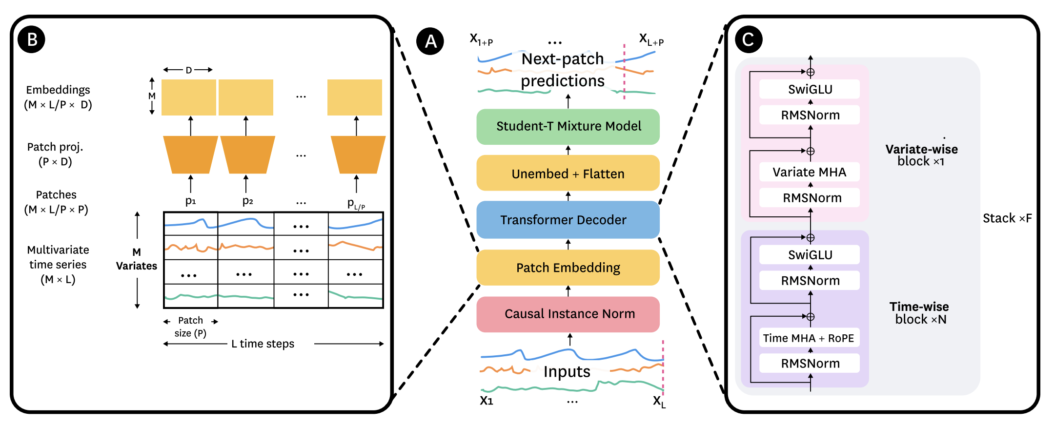
Code for the Toto v1 model can be found here. The v1 release is open weights and is used along with our production Toto configuration. We target NVIDIA A10 inference performance on Float32 data.
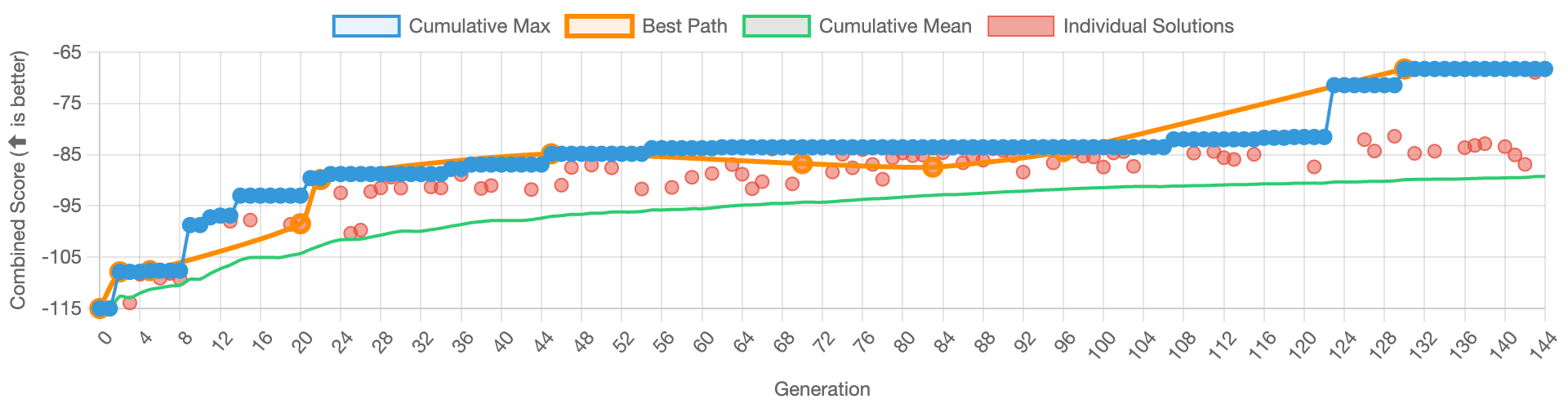
BitsEvolve produced an optimized implementation that achieves a 1.57x speedup. The score progression graph is visualized below over 140 generations. Individual candidates are plotted in red and the cumulative mean/max scores are plotted in green and blue respectively. "Best Path" traces the lineage of the best performing candidate. The step function increases in score correlate with one or more significant optimizations, for example a fused kernel that compiles and produces correct results (possibly iterating over multiple generations), or a crossover that incorporates multiple composable optimizations.
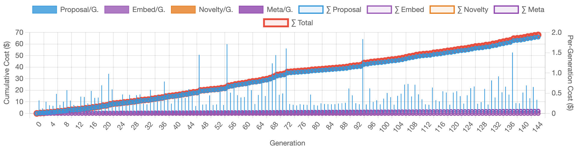
The cost progression below tracks how the workflow performs against the budget cap ($70). The spikes correlate with full rewrites and crossovers, where token usage is typically higher.
Toto Backbone
Since TotoBackbone is transformer-based, we see optimizations similar to SDS, specifically operator fusion and data layout changes for SDPA inputs.
Interestingly, the LLM attempts to fuse the last residual add into the previous linear layer. However, profiling data shows that the layout changes required to fuse the add to the linear's GEMM made the fusion suboptimal, so the agent correctly rejected it.
%%{init: {'theme':'base', 'themeVariables': { 'fontSize':'16px'}}}%%
graph LR
    subgraph Initial[" Initial Model (15 operations) "]
    direction TB
    I0[ ]
    I1[RMSNorm: compute x²]
    I2[RMSNorm: mean + rsqrt]
    I3[RMSNorm: scale]
    I4[Compute cos/sin]
    I5[Rotate Q separately]
    I6[Rotate K separately]
    I7[Q·K^T attention<br/>SDPA]
    I8[Residual add]
    I9[RMSNorm: compute x²]
    I10[RMSNorm: mean + rsqrt]
    I11[RMSNorm: scale]
    I12[Linear expand to 2H]
    I13[Chunk into gate/val]
    I14[SiLU + multiply]
    I15[Linear project to D]
    I16[Residual add]
    end

    subgraph Optimized[" Optimized Model (6 operations) "]
    direction TB
    O0[ ]
    O1[Fused RMSNorm<br/>shared memory]
    O2[Fused QK Rotary<br/>time-aware scaling]
    O3[Q·K^T attention<br/>SDPA]
    O4[Fused Add + RMSNorm<br/>dual output]
    O5[Fused MLP<br/>cuBLAS + SwiGLU]
    O6[Residual add]
    end

    I1 -.-> O1
    I2 -.-> O1
    I3 -.-> O1
    I4 -.-> O2
    I5 -.-> O2
    I6 -.-> O2
    I7 -.-> O3
    I8 -.-> O4
    I9 -.-> O4
    I10 -.-> O4
    I11 -.-> O4
    I12 -.-> O5
    I13 -.-> O5
    I14 -.-> O5
    I15 -.-> O5
    I16 -.-> O6

    style I0 fill:none,stroke:none
    style O0 fill:none,stroke:none
    style O1 fill:#51cf66,color:#fff
    style O2 fill:#51cf66,color:#fff
    style O4 fill:#51cf66,color:#fff
    style O5 fill:#51cf66,color:#fff
Toto Forecaster
On the forecaster side, BitsEvolve generates
- A fused kernel for the affine transform + KV cache write.
- Basic optimizations around tensor accesses and indexing (improving speed without custom CUDA code).
- A zero-copy setup phase, which contributes to the overall speedup.
graph TB
    subgraph "TotoForecaster.forecast()"
    direction TB
    A[Input Time Series] --> B[Setup Phase<br/>Zero-copy expand]
    B --> C[Autoregressive Loop<br/>N steps]

    subgraph "Each Step"
    C1[Model Forward Pass] --> C2[Sample Distribution]
    C2 --> C3[Fused Affine+Write]
    end

    C --> C1
    C3 --> C4{More steps?}
    C4 -->|Yes| C1
    C4 -->|No| D[Return Samples]
    end

    subgraph "Model Forward Pass Detail"
    M1[Fused RMSNorm] --> M2[Fused QK Rotary]
    M2 --> M3[SDPA Attention]
    M3 --> M4[Fused Add+RMSNorm]
    M4 --> M5[Fused MLP]
    M5 --> M6[Output Distribution]
    end

    C1 -.-> M1
    M6 -.-> C2

    style B fill:#51cf66,color:#fff
    style C3 fill:#51cf66,color:#fff
    style M1 fill:#51cf66,color:#fff
    style M2 fill:#51cf66,color:#fff
    style M4 fill:#51cf66,color:#fff
    style M5 fill:#51cf66,color:#fff
Optimized Code Example: Toto Rotary Embedding
Reference PyTorch Code
def apply_rotary_emb(
    freqs,
    t,
    start_index=0,
    scale=1.,
    seq_dim=-2,
    freqs_seq_dim=None
):
    """
    Apply rotary embeddings (from rotary_embedding_torch library).

    Args:
        freqs: Frequency tensor
        t: Input tensor to apply rotation to
        start_index: Starting index for rotation
        scale: Scaling factor (for xpos)
        seq_dim: Sequence dimension
        freqs_seq_dim: Frequency sequence dimension
    """
    dtype = t.dtype

    if not exists(freqs_seq_dim):
        if freqs.ndim == 2 or t.ndim == 3:
            freqs_seq_dim = 0

    if t.ndim == 3 or exists(freqs_seq_dim):
        seq_len = t.shape[seq_dim]
        freqs = slice_at_dim(freqs, slice(-seq_len, None), dim=freqs_seq_dim)

    rot_dim = freqs.shape[-1]
    end_index = start_index + rot_dim

    assert rot_dim <= t.shape[-1], f'feature dimension {t.shape[-1]} is not of sufficient size to rotate in all the positions {rot_dim}'

    # Split t into three parts: left, middle (to be transformed), and right
    t_left = t[..., :start_index]
    t_middle = t[..., start_index:end_index]
    t_right = t[..., end_index:]

    # Apply rotary embeddings
    t_transformed = (t_middle * freqs.cos() * scale) + (rotate_half(t_middle) * freqs.sin() * scale)

    out = torch.cat((t_left, t_transformed, t_right), dim=-1)

    return out.type(dtype)

def rotate_queries_and_keys(
        self,
        q: torch.Tensor,
        k: torch.Tensor,
        seq_dim: int = None,
        seq_pos_offset: int = 0,
    ):
        """
        Apply rotary embeddings with xpos scaling to queries and keys.
        Uses exact logic from rotary_embedding_torch library.
        """
        if seq_dim is None:
            seq_dim = self.default_seq_dim

        device, dtype, seq_len = q.device, q.dtype, q.shape[seq_dim]

        # Get sequence positions
        seq = self.get_seq_pos(seq_len, dtype=dtype, device=device)
        seq = seq + seq_pos_offset

        # Get frequencies and scale
        freqs = self.forward(seq)
        scale = self.get_scale(seq).to(dtype)

        # Apply rotary embeddings using library function
        rotated_q = apply_rotary_emb(freqs, q, scale=scale, seq_dim=seq_dim)
        rotated_k = apply_rotary_emb(freqs, k, scale=scale**-1, seq_dim=seq_dim)

        return rotated_q.type(dtype), rotated_k.type(dtype)
Optimized Code
def apply_fused_qk_rotary_emb(q, k, cos_base, sin_base, scale_base, seq_pos_offset, seq_dim=-2):
    """Apply rotary embeddings to Q and K with an offset-aware fused kernel (prefers in-place)."""
    seq_len = q.shape[seq_dim]
    end_idx = seq_pos_offset + seq_len

    # OPT: Slice precomputed tables to current sequence window
    cos_freq = cos_base[seq_pos_offset:end_idx].contiguous()
    sin_freq = sin_base[seq_pos_offset:end_idx].contiguous()
    scale = scale_base[seq_pos_offset:end_idx].contiguous()

    if (
        _fused_rotary_inplace_ext is not None
        and q.is_cuda
        and k.is_cuda
        and q.dtype in (torch.float16, torch.float32)
        and q.shape == k.shape
    ):
        _fused_rotary_inplace_ext.fused_qk_rotary_emb_inplace(q.contiguous(), k.contiguous(), cos_freq, sin_freq, scale)
        return q, k

    # OPT: Single fused kernel
    if (
        _fused_rotary_ext is not None
        and q.is_cuda
        and k.is_cuda
        and q.dtype in (torch.float16, torch.float32)
        and q.shape == k.shape
    ):
        return _fused_rotary_ext.fused_qk_rotary_emb_forward(
            q.contiguous(), k.contiguous(), cos_base, sin_base, scale_base, seq_pos_offset
        )

    # Fallback pure PyTorch path
    dtype = q.dtype
    rotated_q = (q * cos_freq + rotate_half(q) * sin_freq) * scale
    rotated_k = (k * cos_freq + rotate_half(k) * sin_freq) * (scale**-1)
    return rotated_q.type(dtype), rotated_k.type(dtype)
template<typename T>
__global__ void fused_qk_rotary_emb_kernel(
    const T* __restrict__ q_in,
    const T* __restrict__ k_in,
    T* __restrict__ q_out,
    T* __restrict__ k_out,
    const T* __restrict__ cos_base,
    const T* __restrict__ sin_base,
    const T* __restrict__ scale_base,
    const int total_pairs,
    const int seq_len,
    const int dim,
    const int seq_pos_offset
) {
    for (int idx = blockIdx.x * blockDim.x + threadIdx.x; idx < total_pairs; idx += gridDim.x * blockDim.x) {
        const int pair_idx_in_token = idx % (dim / 2);
        const int token_idx = idx / (dim / 2);
        const int seq_idx = token_idx % seq_len;
        const int effective_seq_idx = seq_idx + seq_pos_offset;

        const int base_in_idx = token_idx * dim;
        const int freq_idx = effective_seq_idx * dim + 2 * pair_idx_in_token;

        const float c = static_cast<float>(cos_base[freq_idx]);
        const float s = static_cast<float>(sin_base[freq_idx]);
        const float sc_q = static_cast<float>(scale_base[freq_idx]);
        const float sc_k = 1.0f / sc_q;

        // Q
        const float q1 = static_cast<float>(q_in[base_in_idx + 2 * pair_idx_in_token]);
        const float q2 = static_cast<float>(q_in[base_in_idx + 2 * pair_idx_in_token + 1]);
        q_out[base_in_idx + 2 * pair_idx_in_token]     = static_cast<T>((q1 * c - q2 * s) * sc_q);
        q_out[base_in_idx + 2 * pair_idx_in_token + 1] = static_cast<T>((q2 * c + q1 * s) * sc_q);

        // K
        const float k1 = static_cast<float>(k_in[base_in_idx + 2 * pair_idx_in_token]);
        const float k2 = static_cast<float>(k_in[base_in_idx + 2 * pair_idx_in_token + 1]);
        k_out[base_in_idx + 2 * pair_idx_in_token]     = static_cast<T>((k1 * c - k2 * s) * sc_k);
        k_out[base_in_idx + 2 * pair_idx_in_token + 1] = static_cast<T>((k2 * c + k1 * s) * sc_k);
    }
}

std::vector<torch::Tensor> fused_qk_rotary_emb_forward(
    torch::Tensor q,
    torch::Tensor k,
    torch::Tensor cos_base,
    torch::Tensor sin_base,
    torch::Tensor scale_base,
    int seq_pos_offset
) {
    ...
    const int total_pairs = (q.numel() / dim) * (dim / 2);
    auto q_out = torch::empty_like(q);
    auto k_out = torch::empty_like(k);

    if (total_pairs == 0) {
        return {q_out, k_out};
    }

    const int block_size = 256;
    const int num_blocks = (total_pairs + block_size - 1) / block_size;
    const cudaStream_t stream = at::cuda::getCurrentCUDAStream();

    AT_DISPATCH_FLOATING_TYPES_AND_HALF(q.scalar_type(), "fused_qk_rotary_emb_kernel", [&] {
        fused_qk_rotary_emb_kernel<scalar_t><<<num_blocks, block_size, 0, stream>>>(
            q.data_ptr<scalar_t>(),
            k.data_ptr<scalar_t>(),
            q_out.data_ptr<scalar_t>(),
            k_out.data_ptr<scalar_t>(),
            cos_base.data_ptr<scalar_t>(),
            sin_base.data_ptr<scalar_t>(),
            scale_base.data_ptr<scalar_t>(),
            total_pairs,
            seq_len,
            dim,
            seq_pos_offset
        );
    });
    C10_CUDA_KERNEL_LAUNCH_CHECK();
    return {q_out, k_out};
}
What's Next
For all the models mentioned in this blog post, the optimizations have been tested in our production environment and integrated with the serving codebase.
- SDS: We are working with the model team on end-to-end evaluations to enable the optimized model by default.
- Toto: The optimized model is currently serving forecasting requests in production. We plan to expand optimization to L4 targets.
Going forward, we plan to further improve our approach. We want to converge towards high-quality optimizations quickly by leveraging more detailed and fine-grained telemetry and persisting learnings across runs.
The AI-Driven Research Systems (ADRS) initiative is an open, collaborative effort to explore how AI can accelerate scientific discovery itself, from evolving algorithms to optimizing real-world systems.
If you've built, optimized, or experimented with AI-driven research tools, we'd love to hear from you. Share your experiences, insights, or case studies with us in the ADRS Blog Series.
👉 Reach out to us via email: ucbskyadrs@gmail.com
💬 Join us: join.slack.com/t and Discord
If you have any questions, reach out to jai.menon@datadoghq.com!